In this post, I will analyse the Tidytuesday Dataset about a video game from the Steam store using R and Rstudio.
Load the packages
1
2
3
4
5
6
|
library(tidyverse)
library(lubridate)
library(magrittr)
library(ggthemr)
library(RColorBrewer)
library(gganimate)
|
Load the data
1
2
|
video_game <-
  read_csv("https://raw.githubusercontent.com/rfordatascience/tidytuesday/master/data/2019/2019-07-30/video_games.csv")
|
Lets take a look at our dataframe.
 1
 2
 3
 4
 5
 6
 7
 8
 9
10
11
12
|
# A tibble: 6 x 10
  number game  release_date price owners developer publisher
   <dbl> <chr> <chr>        <dbl> <chr>  <chr>     <chr>
1      1 Half… Nov 16, 2004  9.99 10,00… Valve     Valve
2      3 Coun… Nov 1, 2004   9.99 10,00… Valve     Valve
3     21 Coun… Mar 1, 2004   9.99 10,00… Valve     Valve
4     47 Half… Nov 1, 2004   4.99 5,000… Valve     Valve
5     36 Half… Jun 1, 2004   9.99 2,000… Valve     Valve
6     52 CS2D  Dec 24, 2004 NA    1,000… Unreal S… Unreal S…
# … with 3 more variables: average_playtime <dbl>,
#   median_playtime <dbl>, metascore <dbl>
|
 1
 2
 3
 4
 5
 6
 7
 8
 9
10
11
12
13
14
15
16
17
18
19
20
21
22
23
24
25
26
27
28
29
30
31
32
|
     number         game           release_date
 Min.   :   1   Length:26688       Length:26688
 1st Qu.: 821   Class :character   Class :character
 Median :2356   Mode  :character   Mode  :character
 Mean   :2904
 3rd Qu.:4523
 Max.   :8846

     price            owners           developer
 Min.   :  0.490   Length:26688       Length:26688
 1st Qu.:  2.990   Class :character   Class :character
 Median :  5.990   Mode  :character   Mode  :character
 Mean   :  8.947
 3rd Qu.:  9.990
 Max.   :595.990
 NA's   :3095
  publisher         average_playtime   median_playtime
 Length:26688       Min.   :   0.000   Min.   :   0.00
 Class :character   1st Qu.:   0.000   1st Qu.:   0.00
 Mode  :character   Median :   0.000   Median :   0.00
                    Mean   :   9.057   Mean   :   5.16
                    3rd Qu.:   0.000   3rd Qu.:   0.00
                    Max.   :5670.000   Max.   :3293.00
                    NA's   :9          NA's   :12
   metascore
 Min.   :20.00
 1st Qu.:66.00
 Median :73.00
 Mean   :71.89
 3rd Qu.:80.00
 Max.   :98.00
 NA's   :23838
|
video_game dataframe has 26688 rows and 10 columns.
Missing value
Lets check for the missing value in the dataframe.
1
|
colSums(is.na(video_game))
|
1
2
3
4
5
6
|
          number             game     release_date            price
               0                3                0             3095
          owners        developer        publisher average_playtime
               0              151               95                9
 median_playtime        metascore
              12            23838
|
Above output shows that We have missing value in this data frame. We will use the median value to replace the missing value of numerical columns.
 1
 2
 3
 4
 5
 6
 7
 8
 9
10
11
12
13
14
15
16
17
18
19
20
21
22
23
24
25
26
27
28
29
30
|
video_game <- video_game %>% mutate(metascore = replace(
  metascore,
  is.na(metascore),
  median(metascore, na.rm = TRUE)
))

video_game <- video_game %>% mutate(price = replace(
  price,
  is.na(price),
  median(price, na.rm = TRUE)
))

video_game <- video_game %>% mutate(average_playtime = replace(
  average_playtime,
  is.na(average_playtime),
  median(average_playtime, na.rm = TRUE)
))

video_game <- video_game %>% mutate(median_playtime = replace(
  median_playtime,
  is.na(median_playtime),
  median(median_playtime, na.rm = TRUE)
))
video_game <- video_game %>% mutate(
  year = year(mdy(release_date)),
  month = month(mdy(release_date), label = TRUE),
  weekday = wday(mdy(release_date), label = TRUE)
)
video_game <- na.omit(video_game)
colSums(is.na(video_game))
|
 1
 2
 3
 4
 5
 6
 7
 8
 9
10
11
12
13
|
             number                game        release_date
                  0                   0                   0
              price              owners           developer
                  0                   0                   0
          publisher    average_playtime     median_playtime
                  0                   0                   0
          metascore                year               month
                  0                   0                   0
            weekday release_date_pretty                 age
                  0                   0                   0
         max_owners          min_owners
                  0                   0
|
We replaced the numerical values with the median of the respective values and dropped the missing rows in publisher and developer column.
1
2
3
4
5
6
7
|
video_game %<>%
  mutate(
    max_owners = str_trim(word(owners, 2, sep = "\\..")),
    max_owners = as.numeric(str_replace_all(max_owners, ",", "")),
    min_owners = str_trim(word(owners, 1, sep = "\\..")),
    min_owners = as.numeric(str_replace_all(min_owners, ",", ""))
  )
|
The owner column has the range of owner of games and the code create max and min owner of the games.
Let’s see the final data frame:
 1
 2
 3
 4
 5
 6
 7
 8
 9
10
11
12
13
|
# A tibble: 6 x 17
  number game  release_date price owners developer publisher
   <dbl> <chr> <chr>        <dbl> <chr>  <chr>     <chr>
1      1 Half… Nov 16, 2004  9.99 10,00… Valve     Valve
2      3 Coun… Nov 1, 2004   9.99 10,00… Valve     Valve
3     21 Coun… Mar 1, 2004   9.99 10,00… Valve     Valve
4     47 Half… Nov 1, 2004   4.99 5,000… Valve     Valve
5     36 Half… Jun 1, 2004   9.99 2,000… Valve     Valve
6     52 CS2D  Dec 24, 2004  5.99 1,000… Unreal S… Unreal S…
# … with 10 more variables: average_playtime <dbl>,
#   median_playtime <dbl>, metascore <dbl>, year <dbl>, month <ord>,
#   weekday <ord>, release_date_pretty <date>, age <dbl>,
#   max_owners <dbl>, min_owners <dbl>
|
Visualization of Data
 1
 2
 3
 4
 5
 6
 7
 8
 9
10
11
12
13
14
15
|
discrete_pal <- c(
  "#fa4234", "#f5b951", "#e8f538", "#52b0f7",
  "#b84ef5", "#4ed1f5", "#45b58e", "#1a1612",
  "#474ccc", "#47cc92", "#a0cc47", "#c96f32"
)
ggthemr("flat")
ggplot(data = video_game %>% group_by(developer) %>%
         tally(sort = TRUE) %>% head(10)) +
  geom_col(aes(x = reorder(developer, n), y = n, fill = n)) +
  labs(
    title = "Developer with most Games", x = NULL, y = "Game Count",
    fill = "Game Count", caption = "by: @diwastha"
  ) +
  theme_minimal() +
  theme(axis.text.x = element_text(angle = 40, hjust = 1))
|

1
2
3
4
5
6
7
8
9
|
ggplot(data = video_game %>% group_by(publisher) %>%
  tally(sort = TRUE) %>% head(10)) +
  geom_col(aes(x = reorder(publisher, n), y = n, fill = n)) +
  labs(
    title = "Publisher with most Games", y = "Game Count", x = NULL,
    fill = "Game Count", caption = "by: @diwastha"
  ) +
  theme_minimal() +
  theme(axis.text.x = element_text(angle = 40, hjust = 1))
|

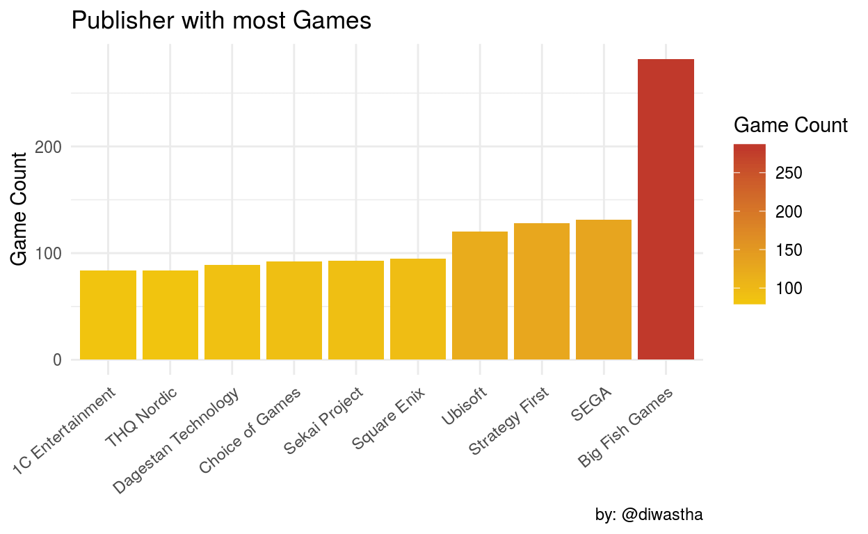
Big Fish Games is the biggest publisher by the game count as it publishes lots of free to play and casual games. Sega which is the second-largest publisher has less than half of the game published by the Big Fish Games.
 1
 2
 3
 4
 5
 6
 7
 8
 9
10
11
12
13
14
15
16
17
18
19
|
video_game %>%
  select(-number) %>%
  mutate(max_owners = as.factor(max_owners / 1000000)) %>%
  group_by(publisher) %>%
  mutate(n = n()) %>%
  ungroup() %>%
  filter(n >= 80) %>%
  ggplot(aes(publisher, max_owners, color = publisher)) +
  geom_jitter(show.legend = FALSE, size = 2, alpha = 0.5) +
  labs(
    title = "Distribution of ownership of top publishers",
    y = "Estimated Game Ownership per Million", x = NULL
  ) +
  theme_minimal() + scale_color_manual(values = discrete_pal) +
  theme(axis.text.x = element_text(angle = 45, hjust = 1)) +
  stat_summary(
    fun.y = mean, geom = "line", shape = 20,
    size = 5, color = "#555555"
  )
|

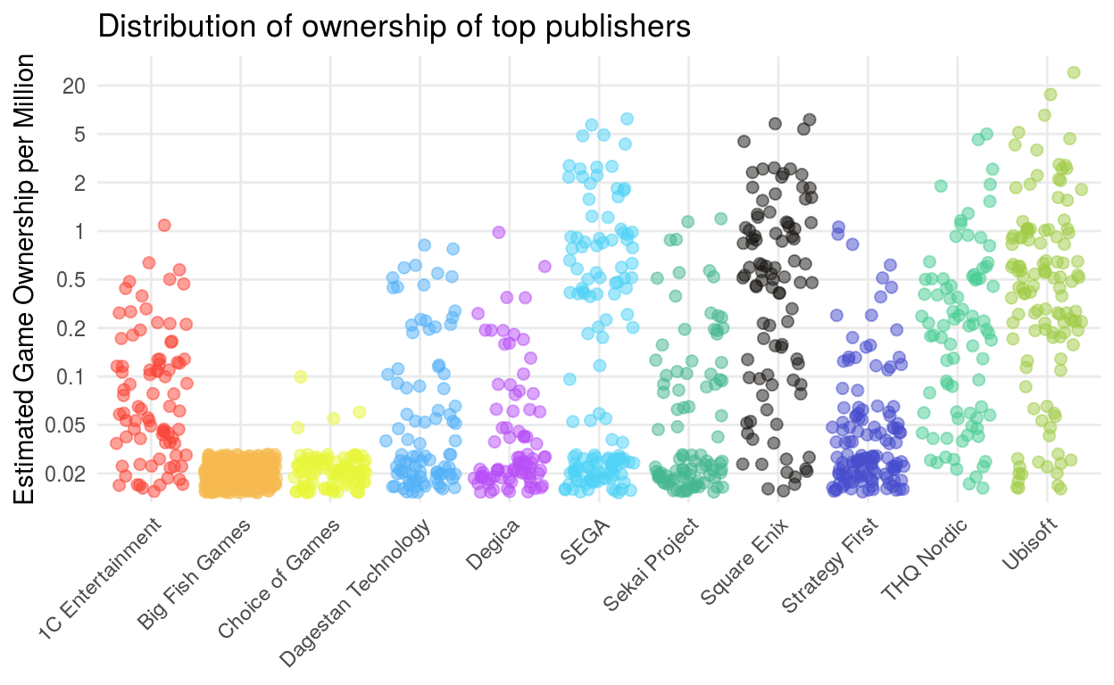
The Big Fish Games has released 265 games but the player base of their games is very small. Other publishers in this group have a much larger player base like Ubisoft, Square Enix, SEGA has much larger player base for their games.
1
2
3
4
5
6
7
8
|
ggplot(data = video_game %>% arrange(desc(average_playtime)) %>% head(20)) +
  geom_col(aes(x = reorder(game, average_playtime), y = average_playtime, fill = metascore)) +
  labs(
    title = "Games with most metascore", x = NULL, y = "Average Playtime",
    caption = "by: @diwastha"
  ) +
  theme_minimal() +
  theme(axis.text.x = element_text(angle = 45, hjust = 1))
|

1
2
3
4
5
6
7
8
9
|
ggplot(data = video_game %>% group_by(max_owners) %>%
         arrange(desc(max_owners)) %>% head(10)) +
  geom_col(aes(x = reorder(game, max_owners), y = max_owners)) +
  labs(
    title = "Most Sold Video Games", y = "Number of copies sold", x = NULL,
    caption = "by: @diwastha"
  ) +
  theme_minimal() +
  theme(axis.text.x = element_text(angle = 45, hjust = 1))
|

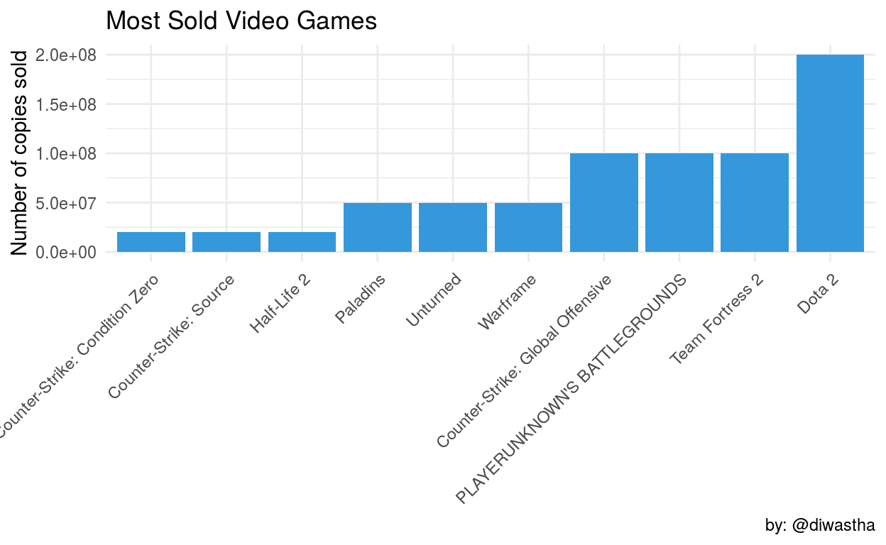
Dota2, Team Fortress 2 is free to play multiplayer games released on 2013 and 2007 respectively. The Player Unknown BattleGround (PUBG) is also a multiplayer battle royale shooter which is a huge hit. Counter-Strike is currently available free in steam which may have increased the owner count. All Top five games are multiplayer games with a strong player base and metascore.
1
2
3
4
5
6
7
8
9
|
ggplot(data = video_game %>% group_by(max_owners) %>%
         arrange(desc(max_owners)) %>% head(10)) +
  geom_col(aes(x = reorder(game, price), y = price, fill = price)) +
  labs(
    title = "Price of most sold games", y = "Price in $", x = NULL,
    caption = "by: @diwastha"
  ) +
  theme_minimal() +
  theme(axis.text.x = element_text(angle = 45, hjust = 1))
|

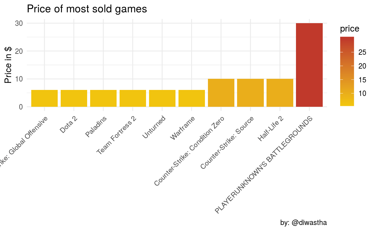
PUBG is currently one of the most popular games in the steam store and huge player base. Other games in this group have a very low price or currently free in the Steam store.
 1
 2
 3
 4
 5
 6
 7
 8
 9
10
11
12
|
ggthemr("flat")
ggplot(
  data = video_game %>% group_by(year) %>%
    summarise(avg_price = mean(price)),
  aes(x = year, y = avg_price)
) +
  geom_line() + geom_point(color = "red") +
  labs(
    title = "Average Price of the Game over the year",
    x = NULL, y = "price in $", caption = "by: @diwastha"
  ) +
  theme_minimal()
|

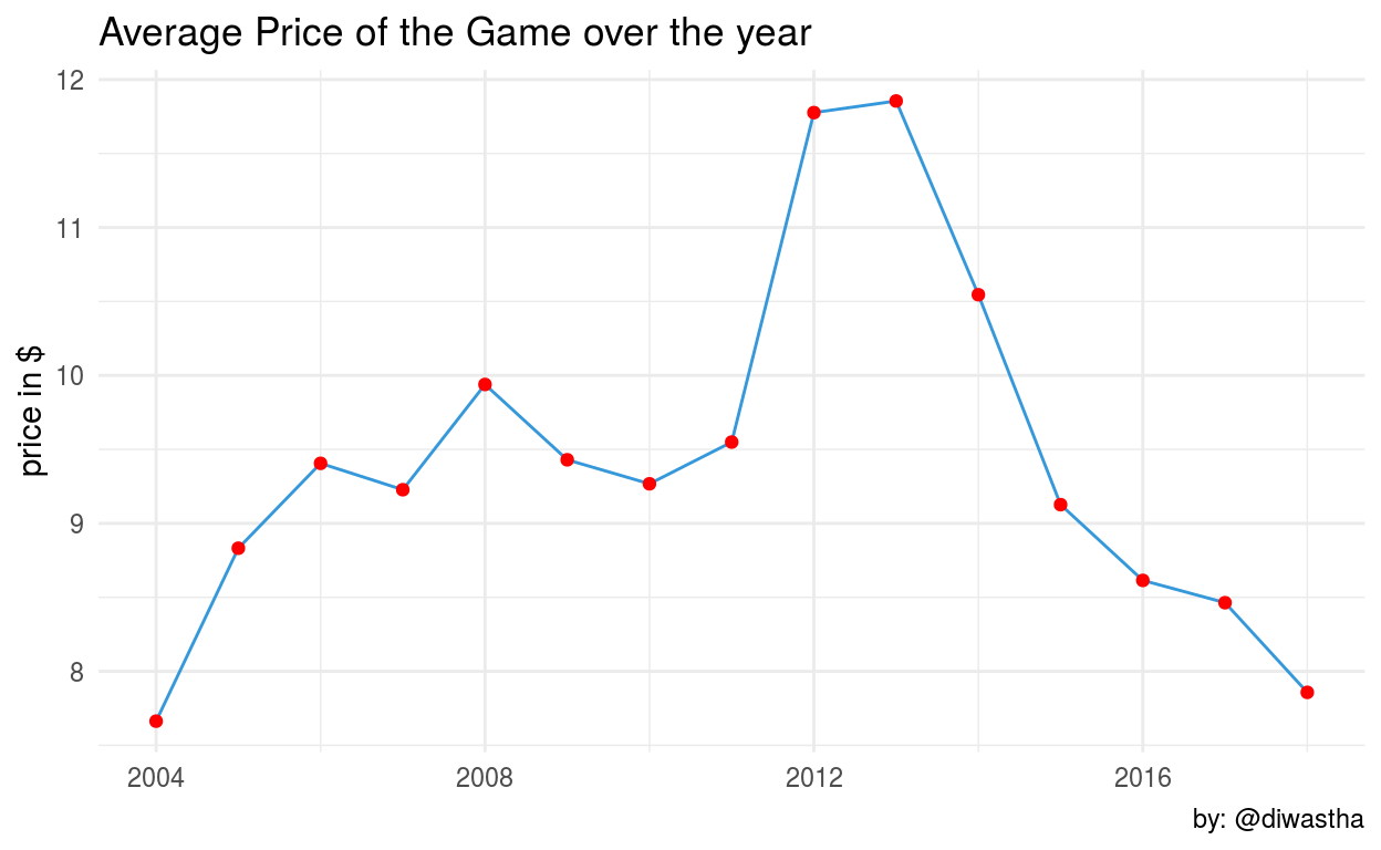
The average game price was rising up to the year 2013 then it started to decrease. It may be due to the increment in the release of the game with a very low price or freemium model.
1
2
3
4
5
6
|
ggplot(data = video_game) + geom_bar(aes(x = year)) +
  labs(
    title = "Number of active games since release year",
    y = "Number of Game", x = NULL, caption = "by: @diwastha"
  ) +
  theme_minimal()
|

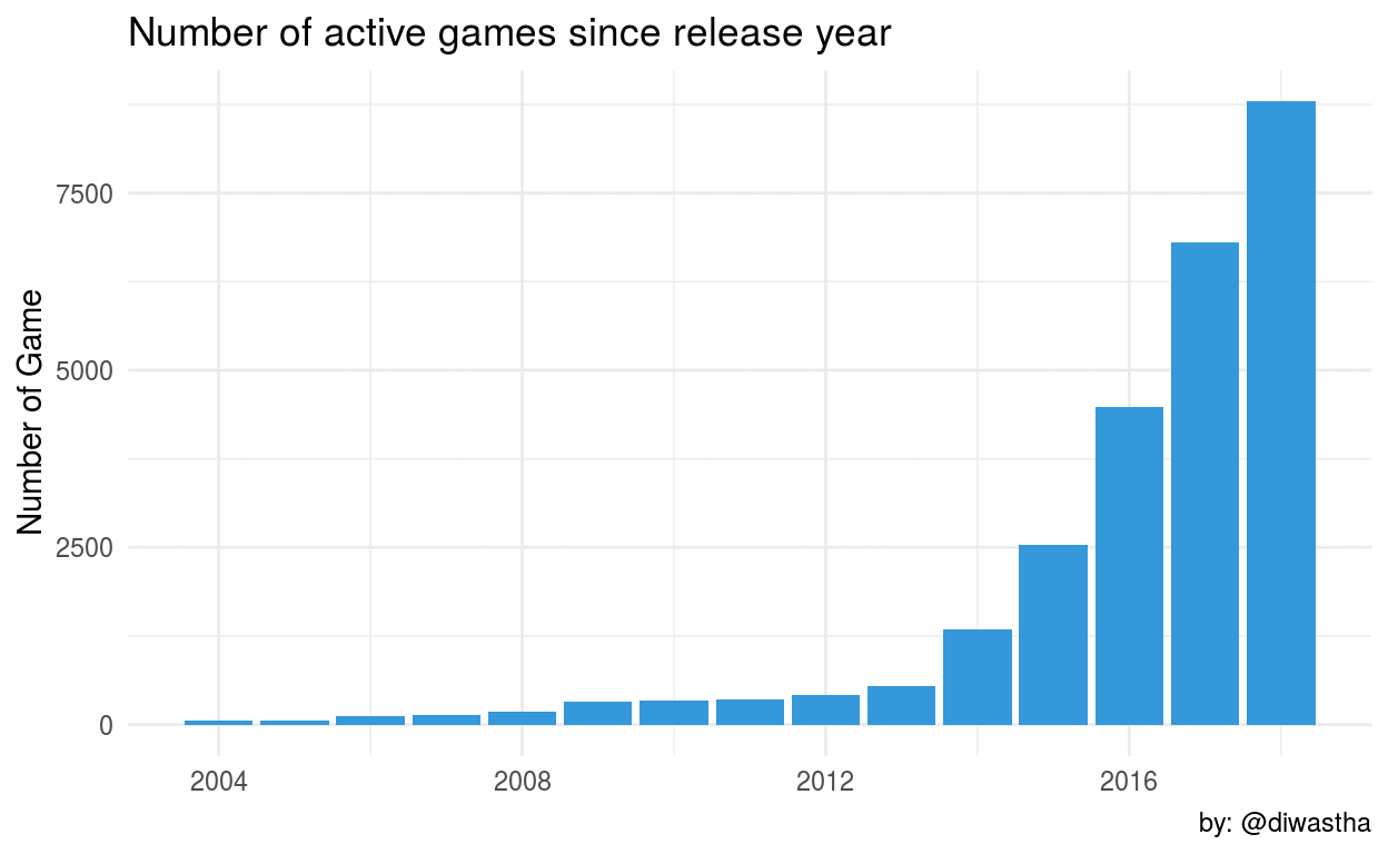
There is growth in the release of the games from the year 2015 onward.
1
2
3
4
5
6
7
8
|
ggplot(data = video_game) + geom_bar(aes(x = month)) +
  transition_time(year) +
  labs(
    title = "Games released in each month",
    subtitle = "Year: {frame_time}",
    y = "Number of Game", x = NULL, caption = "by: @diwastha"
  ) +
  theme_minimal()
|

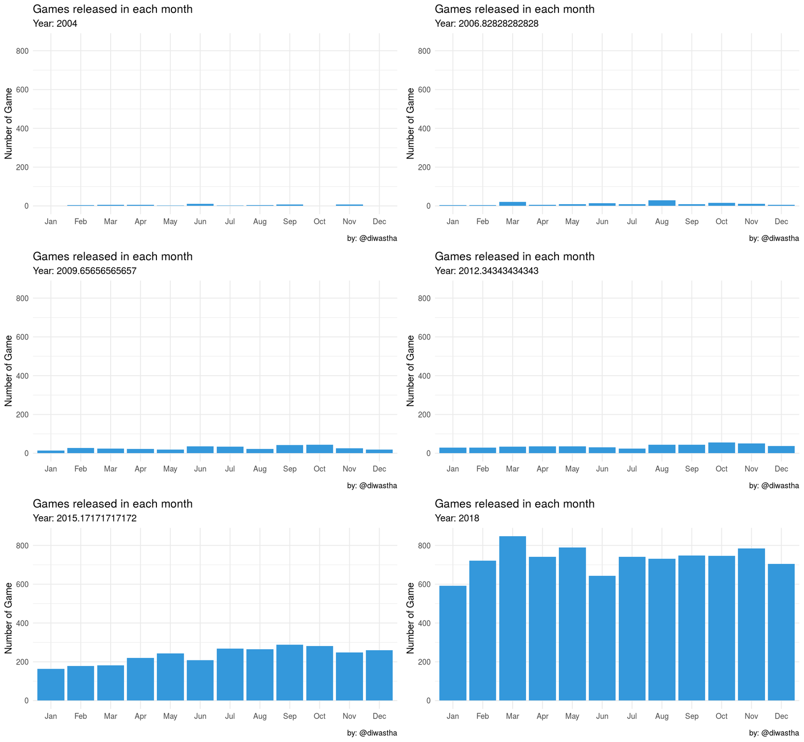
The above animation shows the number of games released on each month of the year.
 1
 2
 3
 4
 5
 6
 7
 8
 9
10
11
12
13
|
ggplot(data = video_game %>% mutate(release_date = mdy(release_date)) %>%
  group_by(release_date) %>%
  summarise(count_games = n()) %>%
  mutate(
    day_of_week = weekdays(release_date),
    weekend = ifelse(day_of_week %in% c("Saturday", "Sunday"),
      "yes",
      "no"
    )
  )) +
  geom_jitter(aes(x = release_date, y = count_games, color = weekend), alpha = 0.4) +
  labs(title = "Games released on weekend", y = "Number of Games", x = NULL) +
  theme_minimal()
|

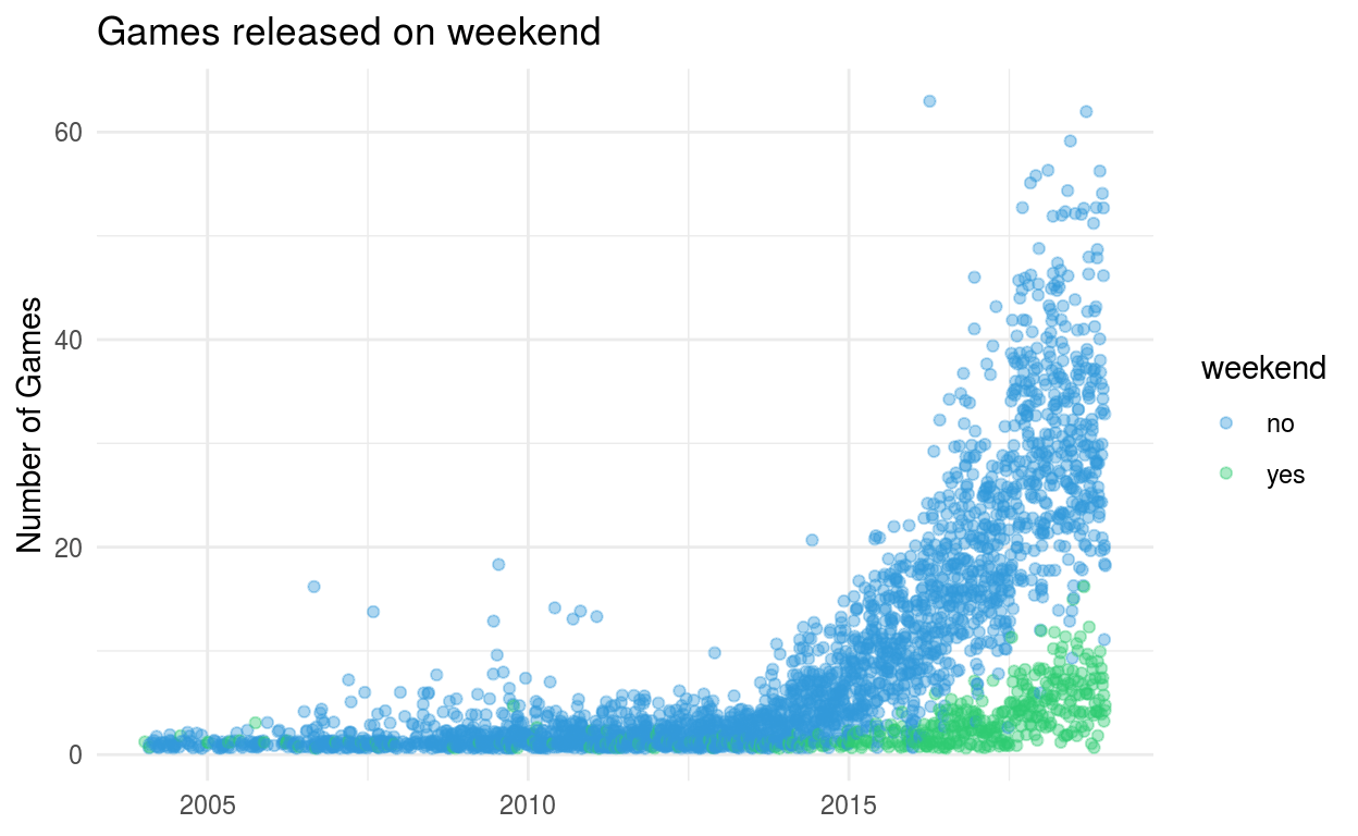
There is a rise in the release of games since 2015 and much of the games are released on workdays than the weekend days.
Wrapping up
Tidytuesday repo has a great dataset for analysis and visualization. You can also extract other data from the repo and work on it. I have taken some references from the work of other people while working on this data and they are:

